Measurement error
- deviation of the measured value of a quantity from its true (actual) value. Measurement error is a characteristic of measurement accuracy.
It is, as a rule, impossible to determine with absolute accuracy the true value of the measured value, and therefore it is impossible to indicate the amount of deviation of the measured value from the true one. This deviation is usually called measurement error
.[1] It is only possible to estimate the magnitude of this deviation, for example, using statistical methods.
In practice, instead of the true value the actual value of the quantity x
d is used, that is, the value of a physical quantity obtained experimentally and so close to the true value that in the given measurement task it can be used instead [1].
This value is usually calculated as the average value obtained from statistical processing of the results of a series of measurements. This obtained value is not exact, but only the most probable. Therefore, when recording measurement results, it is necessary to indicate their accuracy. For example, recording T
= 2.8 ± 0.1 s;
P = 0.95 means that the true value of T
lies in the range from
2.7 s
to
2.9 s
with a confidence level of 95%.
Quantifying the magnitude of measurement error—a measure of “doubt about the quantity being measured”—leads to the concept of “measurement uncertainty.” At the same time, sometimes, especially in physics, the term “measurement error” is used as a synonym for the term “measurement uncertainty” [2].
Classification of measurement errors
By way of expression
Absolute error [3] Absolute error is a value expressed in units of the measured value. It can be described by the formula Δ X = X measured − X true. {\displaystyle \Delta X=X_{\text{measured}}-X_{\text{true}}.} Instead of the true value of the measured quantity, in practice they use the actual value X d , {\displaystyle {X_{\text{d} }},} which is close enough to the true one and which is determined experimentally and can be taken instead of the true one. Due to the fact that the true value of a quantity is always unknown, it is only possible to estimate the boundaries within which the error lies, with some probability. This assessment is carried out using the methods of mathematical statistics[4]. Relative error[3] Relative error is expressed by the ratio δ X = Δ XX d. {\displaystyle \delta X={\frac {\Delta X}{X_{\text{d}}}}.} The relative error is a dimensionless quantity; its numerical value can be indicated, for example, as a percentage.
By source of occurrence
Instrumental error[5] This error is determined by the imperfection of the device, arising, for example, due to inaccurate calibration. Methodical error [5] Methodical error is an error caused by imperfection of the measurement method. These include errors from the inadequacy of the adopted model of the object or from the inaccuracy of calculation formulas. Subjective error [5] Subjective error is an error caused by limited capabilities and human errors when making measurements: it manifests itself, for example, in inaccuracies when reading readings from the instrument scale.
By nature of manifestation
Random error This is a component of the measurement error that changes randomly in a series of repeated measurements of the same quantity, carried out under the same conditions.
There is no pattern observed in the appearance of such errors; they are detected during repeated measurements of the same quantity in the form of some scatter in the results obtained. Random errors are inevitable and are always present as a result of measurement, but their influence can usually be eliminated by statistical processing. Description of random errors is possible only on the basis of the theory of random processes and mathematical statistics. Mathematically, random error can usually be represented as white noise: as a continuous random variable, symmetric about zero, occurring independently in each dimension (uncorrelated in time).
The main property of random error is that distortions of the desired value can be reduced by averaging the data. Refining the estimate of the desired value with an increase in the number of measurements (repeated experiments) means that the average random error tends to 0 as the volume of data increases (the law of large numbers).
Often random errors arise due to the simultaneous action of many independent causes, each of which individually has little effect on the measurement result. For this reason, the random error distribution is often assumed to be “normal” (see “Central Limit Theorem”
). “Normality” allows you to use the entire arsenal of mathematical statistics in data processing.
However, the a priori belief in “normality” based on the central limit theorem is not consistent with practice - the laws of distribution of measurement errors are very diverse and, as a rule, differ greatly from normal. [ source not specified 30 days
]
Random errors can be associated with imperfection of instruments (for example, with friction in mechanical devices), with shaking in urban conditions, with imperfection of the measurement object itself (for example, when measuring the diameter of a thin wire, which may not have a completely round cross-section as a result of imperfections in the manufacturing process ).
Systematic error This is an error that varies according to a certain law (in particular, a constant error that does not change from measurement to measurement). Systematic errors may be associated with instrument errors (incorrect scale, calibration, etc.) not taken into account by the experimenter.
Systematic error cannot be eliminated by repeated measurements. It can be eliminated either through corrections or by “improving” the experiment.
The division of errors into random and systematic is quite arbitrary. For example, a rounding error under certain conditions can be of the nature of both a random and systematic error.
Permissible measurement error: selecting a value
V.D.
Gvozdev. Permissible measurement error: choice of value
(“Legislative and Applied Metrology”, 2013, No. 2)
annotation
The object of the analysis is recommendations for the selection of permissible measurement error contained in regulatory documents and publications on metrology. The main attention is paid to tolerance quality control. It is emphasized that the concept of monitoring the accuracy of linear dimensions adopted in GOST 24356 may be the cause of defects.
Keywords:
measurements, control, permissible measurement error, permissible measurement error, tolerance, conformity assessment
To ensure the uniformity of measurements, it is necessary that the characteristics of the error/uncertainty (hereinafter referred to as error - Δ) of the measurement result do not go beyond the specified (permissible) limits. Methods for determining the accuracy characteristics of measurement results are the main topic of metrology. Little attention is paid to the selection of permissible error values. Often the authors of books limit themselves to indicating that the choice of permissible (permissible) error is made based on the measurement tasks. This is due to the fact that within the framework of metrology it is impossible to justify the choice of the permissible error value.
However, it is also impossible to leave the topic of choosing the permissible error without consideration, if only because during the metrological examination of draft regulatory documents, design and technological documentation, the optimality of the requirements for measurement accuracy is necessarily checked.
The task of measurements is to determine the value of a quantity. Goals may be different. Let's divide them conditionally into two groups: 1 - obtaining information about the size and 2 - monitoring the quality of objects.
In the first case, the values of the permissible measurement error are determined by the influence of the uncertainty of the measurement result on the consequences of making a decision based on it.
For example:
- if the task is to increase the accuracy of the assessment of any quantitative characteristic in relation to the already achieved level, the permissible measurement error will be determined by the digit of the last digit, the reliability of which must be ensured;
- for scientific and practical research, in many cases, the permissible measurement error is established based on the condition of comparability of their results;
- in medicine, the accuracy of measurements is determined by the relationship between the change in the parameter and the patient’s well-being;
- in sports, the choice of resolution of measuring instruments and measurement errors are associated with the density of athletes’ results;
- when carrying out trade operations with products characterized by mass or volume, supply of electricity, heat, fuels and lubricants, etc., the economic indicators of the supplier and consumer directly depend on the value of the permissible measurement error;
- when assessing the accuracy characteristics of technological processes, applying statistical methods for monitoring technological processes, statistical acceptance control and incoming product quality control, they proceed from the criterion of negligible measurement error in relation to the technological tolerance. The measurement accuracy characteristics are taken such that the standard deviation (RMSD) of the measurement result is 5...6 times less than the standard deviation of the controlled parameter [1]. If the standard deviation of the controlled parameter is unknown, they are guided by the rule: the division value should not exceed 1/6 of the tolerance value of the controlled parameter [2]. The measurement error in this case is considered as an integral part of the manufacturing error.
When establishing requirements for the quality of objects, one-sided restrictions or two-sided restrictions (tolerances) are set for the values of quality indicators, which are taken into account when choosing the permissible measurement error. Let us determine the location of the measurement error when monitoring a quality indicator with a two-sided constraint, that is, when a tolerance is specified. Let us turn to the provision written in the GOST R ISO 10576-1-2006 standard [3]: “a decision on compliance with the requirements can be made if the uncertainty interval of the measurement results is within the range of permissible values.” Implementing the principles of conformity assessment established by the standard, we will depict the areas of compliance (the controlled parameter A is clearly within the specified limits) and non-compliance (the controlled parameter A is clearly outside the specified limits) on the numerical axis (Fig.).
Rice. Scheme of measuring quality control of a separate object.
Compliance area 1 is defined by the condition Аmin + Δ ≤ А ≤ Аmax – Δ, areas of non-compliance 2 (areas of unacceptable values) are characterized by the inequalities А ≤ Аmin – Δ and A ≥ Аmax + Δ. We will call the intervals Amin ± Δ and Amax ± Δ the areas of the inconclusive result of the conformity assessment 3. If the true value of the measured value is in the area of the inconclusive result of the conformity assessment, then there is a possibility that, due to the influence of measurement error, a suitable product may be classified as defective (incorrectly rejected product) , and the defective product becomes acceptable (wrongly accepted product).
With a known distribution function 4 of the measurement error, it is possible to establish the probabilities of correct and incorrect decisions about the conformity of a particular
product.
In relation to the situation shown in the figure, if A* is the true value of the quantity, then Pr is the probability of recognizing the product as suitable, and Pb = 1- Pr is the probability of rejecting the product. If A* is a measured value, then Pr is the probability that the product is good, and Pb is the probability that it is defective. The reliability of such information is not high: information about the law of distribution of random measurement error is approximate or absent; non-excluded systematic errors, considered when calculating the total error as random variables, in practical measurements manifest themselves as systematic components, the values and signs of which are unknown.
Standard [3] does not provide rules for the situation when an inconclusive conformity assessment result is obtained. At the same time, about making wrong decisions. The two-step procedure involves repeating measurements when the uncertainty interval calculated after the first step falls outside the tolerance range (i.e. the measurement result is in the area of the inconclusive conformity assessment result). The value of the measured quantity and its uncertainty are established as a combination of the measurement results of two stages.
To bring closer the boundaries of the area of inconclusive conformity assessment results, measures to reduce measurement errors discussed in document [4] are applicable.
The boundaries of the compliance area are narrowed to zero when the permissible measurement error is equal to 0.5 of the manufacturing tolerance and expand to the boundaries of the tolerance area in the absence of measurement error. It follows from this that the value of the measurement error with a two-sided limitation of the quality indicator should be less than half the tolerance value
and the smaller it is, the better.
The conclusion is consistent with the opinion of the authors of [5, 6] and this is the only
general
recommendation that is advisable to give within the framework
of metrology
.
Regulatory documents and printed publications on metrology provide other guidelines for choosing the permissible measurement error, which supposedly allow “to achieve the required accuracy of products with the least amount of labor and material costs” [7].
Page 1 of 3 Next
Estimation of error in direct measurements
In direct measurements, the required value is determined directly from the reading device (scale) of the measuring instrument. In general, measurements are carried out according to a certain method and using certain measuring instruments. These components are imperfect and contribute to measurement error[6]. If in one way or another the measurement error (with a specific sign) can be found, then it represents a correction that is simply excluded from the result. However, it is impossible to achieve an absolutely accurate measurement result, and some “uncertainty” always remains, which can be identified by estimating the error limits [7]. In Russia, methods for assessing error in direct measurements are standardized by GOST R 8.736-2011[8] and R 50.2.038-2004[9].
Depending on the available source data and the properties of the errors that are being assessed, various assessment methods are used. The random error, as a rule, obeys the law of normal distribution, to find which it is necessary to indicate the mathematical expectation M {\displaystyle M} and the standard deviation σ. {\displaystyle \sigma .} Due to the fact that a limited number of observations are carried out during the measurement, only the best estimates of these quantities are found: the arithmetic mean (that is, the final analogue of the mathematical expectation) of the observation results x ¯ {\displaystyle {\bar {x} }} and standard deviation of the arithmetic mean S x ¯ {\displaystyle S_{\bar {x}}} [10][8]:
x ¯ = ∑ i = 1 nxin {\displaystyle {\bar {x}}={\frac {\sum _{i=1}^{n}x_{i}}{n}}} ; S x ¯ = ∑ i = 1 n ( xi − x ¯ ) 2 n ( n − 1 ) . {\displaystyle S_{\bar {x}}={\sqrt {\frac {\sum _{i=1}^{n}(x_{i}-{\bar {x}})^{2}} {n(n-1)}}}.}
The confidence limits ε {\displaystyle \varepsilon } of the error estimate obtained in this way are determined by multiplying the standard deviation by the Student coefficient t, {\displaystyle t,} chosen for a given confidence probability P: {\displaystyle P:}
ε = t S x ¯ . {\displaystyle \varepsilon =tS_{\bar {x}}.}
Systematic errors, by virtue of their definition, cannot be assessed through repeated measurements [11]. For the components of a systematic error due to the imperfection of measuring instruments, as a rule, only their boundaries are known, represented, for example, by the main error of the measuring instrument [12].
The final estimate of the error limits is obtained by summing up the above “elementary” components, which are considered as random variables. This problem can be solved mathematically with known distribution functions of these random variables. However, in the case of a systematic error, such a function is usually unknown and the shape of the distribution of this error is set as uniform [13]. The main difficulty lies in the need to construct a multidimensional distribution law for the sum of errors, which is practically impossible even with 3-4 components. Therefore, approximate formulas are used [14].
The total non-excluded systematic error, when it consists of several m {\displaystyle m} components, is determined by the following formulas[8]:
Θ ∑ = ± ∑ i = 1 m | Θ i | {\displaystyle \Theta _{\sum }=\pm \sum _{i=1}^{m}\left|\Theta _{i}\right|} (if m < 3 {\displaystyle m<3} ); Θ ∑ ( P ) = ± k ∑ i = 1 m Θ i 2 {\displaystyle \Theta _{\sum }(P)=\pm k{\sqrt {\sum _{i=1}^{m}\ Theta _{i}^{2}}}} (if m ⩾ 3 {\displaystyle m\geqslant 3}), where the coefficient k {\displaystyle k} for the confidence probability P = 0, 95 {\displaystyle P=0{ ,}95} is equal to 1.1.
The total measurement error, determined by the random and systematic components, is estimated as [15][8]:
Δ = KS x ¯ 2 + Θ ∑ 2 3 {\displaystyle \Delta =K{\sqrt {S_{\bar {x}}^{2}+{\frac {\Theta _{\sum }^{2} }{3}}}}} or Δ = KS x ¯ 2 + ( Θ ∑ ( P ) k 3 ) 2 {\displaystyle \Delta =K{\sqrt {S_{\bar {x}}^{2}+ \left({\frac {\Theta _{\sum }(P)}{k{\sqrt {3}}}}\right)^{2}}}} , where K = ε + Θ ∑ S x ¯ + Θ ∑ 3 {\displaystyle K={\frac {\varepsilon +\Theta _{\sum }}{S_{\bar {x}}+{\frac {\Theta _{\sum }}{\sqrt { 3}}}}}} or K = ε + Θ ∑ ( P ) S x ¯ + Θ ∑ ( P ) k 3 . {\displaystyle K={\frac {\varepsilon +\Theta _{\sum }(P)}{S_{\bar {x}}+{\frac {\Theta _{\sum }(P)}{k {\sqrt {3}}}}}}.}
The final measurement result is written as[16][8][17][18] A ± Δ ( P ) , {\displaystyle A\pm \Delta (P),} where A {\displaystyle A} is the measurement result ( x ¯ , {\displaystyle {\bar {x}},} ) Δ {\displaystyle \Delta } - confidence limits of the total error, P {\displaystyle P} - confidence probability.
Standardization of errors of measuring instruments
Standardization of errors of measuring instruments
Standardization of metrological characteristics of measuring instruments consists in establishing boundaries for deviations of the real values of the parameters of measuring instruments from their nominal values.
Each measuring instrument is assigned certain nominal characteristics. The actual characteristics of measuring instruments do not coincide with the nominal ones, which determines their errors.
Usually the normalizing value is taken equal to:
- the greater of the measurement range if the zero mark is located at the edge or outside the measurement range;
- the sum of the modules of the measurement limits, if the zero mark is located inside the measurement range;
- the length of the scale or its part corresponding to the measurement range, if the scale is significantly uneven (for example, with an ohmmeter);
- the nominal value of the measured quantity, if one is established (for example, for a frequency meter with a nominal value of 50 Hz);
- module of the difference in measurement limits, if a scale with a conditional zero is adopted (for example, for temperature), etc.
Most often, the upper measurement limit of a given measuring instrument is taken as the normalizing value.
Deviations of the parameters of measuring instruments from their nominal values, causing measurement errors, cannot be indicated unambiguously, therefore maximum permissible values must be established for them.
The specified standardization is a guarantee of the interchangeability of measuring instruments.
Standardization of errors of measuring instruments consists of establishing a limit of permissible error.
This limit is understood as the largest (without taking into account the sign) error of a measuring instrument, at which it can be considered suitable and allowed for use.
The approach to normalizing the errors of measuring instruments is as follows:
- standards indicate the limits of permissible errors, which include both systematic and random components;
- separately standardize all properties of measuring instruments that affect their accuracy.
The standard establishes a series of limits of permissible errors. The same purpose is served by establishing accuracy classes of measuring instruments.
Accuracy classes of measuring instruments
The accuracy class is a generalized characteristic of an SI, expressed by the limits of the permissible values of its main and additional errors, as well as other characteristics that affect the accuracy. The accuracy class is not a direct assessment of the accuracy of measurements performed by this measuring instrument, since the error also depends on a number of factors: measurement method, measurement conditions, etc. The accuracy class only allows one to judge the limits within which the SI error of a given type lies. The general provisions for dividing measuring instruments by accuracy class are established by GOST 8.401–80.
The limits of permissible main error, determined by the accuracy class, are the interval in which the value of the main SI error lies.
SI accuracy classes are established in standards or technical specifications. The measuring instrument may have two or more accuracy classes. For example, if it has two or more measurement ranges of the same physical quantity, it can be assigned two or more accuracy classes. Instruments designed to measure several physical quantities may also have different accuracy classes for each measured quantity.
The limits of permissible main and additional errors are expressed in the form of reduced, relative or absolute errors. The choice of presentation form depends on the nature of the change in errors within the measurement range, as well as on the conditions of use and purpose of the SI.
The limits of the permissible absolute basic error are set according to one of the formulas: or , where x is the value of the measured quantity or the number of divisions counted on the scale; a, b are positive numbers independent of x. The first formula describes a purely additive error, and the second formula describes the sum of additive and multiplicative errors.
In technical documentation, accuracy classes established in the form of absolute errors are designated, for example, “Accuracy class M”, and on the device - with the letter “M”. Capital letters of the Latin alphabet or Roman numerals are used for designation, and smaller error limits should correspond to letters located closer to the beginning of the alphabet or smaller numbers. The limits of the permissible reduced basic error are determined by the formula, where xN is the normalizing value, expressed in the same units as; p is an abstract positive number selected from a range of values:
The normalizing value xN is set equal to the larger of the measurement limits (or modules) for SI with a uniform, almost uniform or power scale and for measuring transducers for which the zero value of the output signal is at the edge or outside the measurement range. For SI, the scale of which has a conventional zero, is equal to the modulus of the difference in measurement limits.
For instruments with a significantly uneven scale, xN is taken equal to the entire length of the scale or its part corresponding to the measurement range. In this case, the limits of absolute error are expressed, like the length of the scale, in units of length, and on the measuring instrument the accuracy class is conventionally indicated, for example, in the form of a symbol, where 0.5 is the value of the number p (Fig. 3.1).
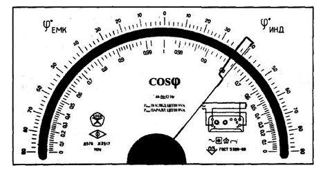
Rice.
3.1. The front panel of a phase meter with an accuracy class of 0.5 with a significantly uneven lower scale
In the remaining cases considered, the accuracy class is designated by a specific number p, for example 1.5. The designation is applied to the dial, shield or body of the device (Fig. 3.2).
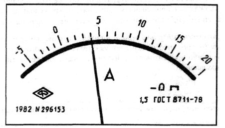
Rice.
3.2. The front panel of an ammeter of accuracy class 1.5 with a uniform scale
In the event that the absolute error is given by the formula, the limits of the permissible relative basic error
| ( 3.1) |
where c, d are abstract positive numbers selected from the series: ; – the largest (in absolute value) of the measurement limits. When using formula 3.1, the accuracy class is indicated in the form “0.02/0.01”, where the numerator is the specific value of the number c, the denominator is the number d (Fig. 3.3).
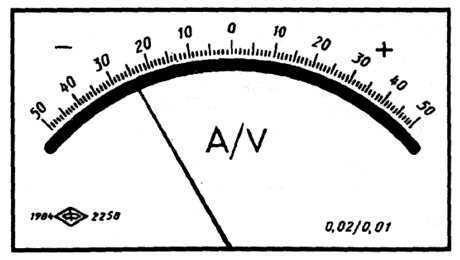
Rice.
3.3. Front panel of ampere-voltmeter accuracy class 0.02/0.01 with uniform scale
The limits of permissible relative main error are determined by the formula, if. The value of the constant number q is set in the same way as the value of the number p. The accuracy class for a device is indicated in the form , where 0.5 is the specific value of q (Fig. 3.4).
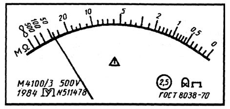
Rice.
3.4. The front panel of a megohmmeter of accuracy class 2.5 with an uneven scale
Standards and technical specifications for SI indicate the minimum value x0, starting from which the accepted method of expressing the limits of permissible relative error is applicable. The ratio xk/x0 is called the dynamic range of the measurement.
Construction rules and examples of designation of accuracy classes in documentation and on measuring instruments are given in Table 3.1.
Table 3.1. Designation of accuracy classes of measuring instruments
| Formula for determining the limits of permissible error | Examples of limits of permissible basic error | Accuracy class designation | |
| In documents | On funds | ||
| Absolute error | |||
| Accuracy class M | M | ||
| Accuracy class C | WITH | ||
| Reduced error | |||
| Accuracy class 1.5 | 1,5 | ||
| Accuracy class 0.5 | (for SI with non-uniform scale) | ||
| Relative error | |||
| Accuracy class 0.5 | |||
| Accuracy class 0.02/0.01 | 0,02/0,01 | ||
Control questions
- Explain what the SI accuracy class is.
- Is the accuracy class of an SI a direct assessment of the accuracy of the measurements performed by this SI?
- List the basic principles underlying the selection of standardized metrological characteristics of measuring instruments.
- How are devices standardized according to accuracy classes?
- What metrological characteristics describe the error of measuring instruments?
- How is the metrological characteristics of measuring instruments regulated?
Measurement error and the Heisenberg uncertainty principle
The Heisenberg uncertainty principle sets a limit on the accuracy of the simultaneous determination of a pair of observable physical quantities that characterize a quantum system and are described by non-commuting operators (for example, position and momentum, current and voltage, electric and magnetic field). Thus, from the axioms of quantum mechanics it follows that it is fundamentally impossible to simultaneously determine certain physical quantities with absolute accuracy. This fact imposes serious restrictions on the applicability of the concept of “true value of a physical quantity” [ source not specified 301 days
].
Maximum measurement error and its components
General information
SELECTION OF UNIVERSAL MEASUREMENT TOOLS FOR ASSESSING LINEAR DIMENSIONS
Errors in measuring instruments (MI) lead to the fact that the measurement result does not correspond to the true size of the part. Due to measurement errors, parts with the correct dimensions may be mistakenly rejected and, conversely, parts with the wrong dimensions are sometimes accepted as acceptable. Parts with incorrect dimensions entering the assembly process result in the production of defective products and can cause significant material damage. To select the correct measuring instrument, it is necessary to be able to assess the influence of measurement errors on the control results.
The influence of measurement errors on the control result is determined by the value of the maximum measurement error. The limits of permissible measurement errors, depending on manufacturing tolerances and nominal measured dimensions, should not exceed the values specified in Table 30 GOST 8.053-81 “Errors allowed when measuring linear dimensions up to 500 mm.”
Table 30 is structured in such a way that for each diameter interval (from the smallest interval up to 3 mm to the largest 400-500 mm) there are 16 rows of limits of permissible measurement errors: from the most accurate row, corresponding to grade 2, to the least accurate - grade 17 In each row, two values are given: the tolerance (IT) for the manufacture of the part (which is taken directly from the drawing of the part under control) and the permissible measurement error (δ).
The principle of choosing measuring instruments is to compare the maximum (total) measurement error Δ∑ with the tabulated permissible measurement error δ. The ratio of these errors to obtain a measurement result with an error no more than a given one must be Δ∑ ≤ δ.
Notes
- ↑ 1 2
In a number of sources, for example in the Great Soviet Encyclopedia, the terms
measurement error
and
measurement error
are used as synonyms, but, according to the recommendation of RMG 29-99, the term
measurement error
, which is considered less successful, is not recommended to be used, and RMG 29-2013 its doesn't mention it at all. See “Recommendations for Interstate Certification 29-2013. GSI. Metrology. Basic terms and definitions." - Olive KA et al.
(Particle Data Group). 38. Statistics. — In: 2014 Review of Particle Physics // Chin. Phys. C. - 2014. - Vol. 38. - P. 090001. - ↑ 12
Friedman, 2008, p. 42. - Friedman, 2008, p. 41.
- ↑ 123
Friedman, 2008, p. 43. - Rabinovich, 1978, p. 19.
- Rabinovich, 1978, p. 22.
- ↑ 1 2 3 4 5
GOST R 8.736-2011 GSI. Multiple direct measurements. Methods for processing measurement results. Basic provisions / VNIIM. — 2011. - R 50.2.038-2004 GSI. Single direct measurements. Estimation of errors and uncertainty of measurement results.
- Rabinovich, 1978, p. 61.
- Friedman, 2008, p. 82.
- Rabinovich, 1978, p. 90.
- Rabinovich, 1978, p. 91.
- Novitsky, 1991, p. 88.
- Rabinovich, 1978, p. 112.
- MI 1317-2004 GSI. Recommendation. Results and characteristics of measurement error. Forms of presentation. Methods of use when testing product samples and monitoring their parameters / VNIIMS. - Moscow, 2004. - 53 p.
- R 50.2.038-2004 Direct single measurements. Estimation of errors and uncertainty of measurement results / VNIIM. - 2011. - 11 p.
- ↑ 12
MI 2083-90 GSI. Indirect measurements, determination of measurement results and estimation of their errors / VNIIM. — 11 s. - Friedman, 2008, p. 129.
Literature
- Yakushev A.I., Vorontsov L.N., Fedotov N.M.
Interchangeability, standardization and technical measurements. — 6th ed., revised. and additional.. - M.: Mashinostroenie, 1986. - 352 p. - Goldin L. L., Igoshin F. F., Kozel S. M. et al.
Laboratory classes in physics. Textbook / ed. Goldina L.L. - M.: Science. Main editorial office of physical and mathematical literature, 1983. - 704 p. - Nazarov N. G.
Metrology. Basic concepts and mathematical models. - M.: Higher School, 2002. - 348 p. — ISBN 5-06-004070-4. - Dedenko L. G., Kerzhentsev V. V.
Mathematical processing and registration of experimental results. - M.: MSU, 1977. - 111 p. — 19,250 copies. - Rabinovich S.G.
Measurement errors. - Leningrad, 1978. - 262 p. - Fridman A.E.
Fundamentals of metrology. Modern course. - St. Petersburg: NPO "Professional", 2008. - 284 p. - Novitsky P.V., Zograf I.A.
Estimation of errors in measurement results. - L.: Energoatomizdat, 1991. - 304 p. — ISBN 5-283-04513-7.